Getting your Dataset ready for Machine Learning

It is important to have a good dataset in addition to a large number of instances to get big results. In this blog post, I am going to focus on preprocessing your raw dataset with python to a format that is ML-friendly.

For now, I am assuming you have a large dataset to play around with.

If you are just starting with machine learning, here are some great public datasets you can use to familiarize yourself with ML concepts.

1. Credit Card default dataset: Can you establish the credibility of a credit card holder? An interesting dataset with over 30,000 records and 24 columns contains information like their age, gender, etc about the credit card holders.
2. Census data: Can you predict whether a person makes over 50k in a year? Census data is a dataset containing over 40000 records and 14 attributes with information about their education, age, work-hours, etc.
3. Hepatitis dataset: Predict the chances of survival of a patient suffering from Hepatitis. This dataset is relatively smaller with 155 records and 19 attributes and contains information about bloodwork, and other symptoms related to this disease.

Now we have our raw dataset, now on to perfecting it. A perfect dataset is like a unicorn of sorts, but thankfully it is neither rare nor elusive. A fine dataset can easily be created with a bit of preprocessing and a bit of understanding what you need from the dataset you have.

If you are working with python, the scikit package is a great package to use for preprocessing your data. If you don't have scikit, no worries. Just install it by copy-pasting the following in your terminal,

pip install scikit-learn

Next, import the package to your code with,

from sklearn import preprocessing

Now, we are set to clean our data, A good way to go about this is to quantify the quality of the data. For this, I am taking the weather dataset as an example, print out the total missing values along with the percentage. This gives you a better idea on which attributes you should be dropping and focusing on.

Total Rows: 142193
              total_missing  perc_missing
Date                       0      0.000000
Location                   0      0.000000
MinTemp                  637      0.447983
MaxTemp                  322      0.226453
Rainfall                1406      0.988797
Evaporation            60843     42.789026
Sunshine               67816     47.692924
WindGustDir             9330      6.561504
WindGustSpeed           9270      6.519308
WindDir9am             10013      7.041838
WindDir3pm              3778      2.656952
WindSpeed9am            1348      0.948007
WindSpeed3pm            2630      1.849599
Humidity9am             1774      1.247600
Humidity3pm             3610      2.538803
Pressure9am            14014      9.855619
Pressure3pm            13981      9.832411
Cloud9am               53657     37.735332
Cloud3pm               57094     40.152469
Temp9am                  904      0.635756
Temp3pm                 2726      1.917113
RainToday               1406      0.988797
RISK_MM                    0      0.000000
RainTomorrow               0      0.000000

Next, for some machine learning algorithms, you need to change the non-numerical data to a numerical format.

You can easily do this with preprocessing package from sklearn. For example, I want to change RainToday which is a non-numerical attribute

Change_number:preprocessing.Labelencoder()
dataset['RainToday'] :Change_number.fit_transform(dataset['RainToday'].astype('str'))

You can easily get a concise summary of your dataset including the type using

dataset.info()

You are almost there with creating the perfect dataset. Often different attributes have a different range, which makes them difficult to compare. A great way to overcome this to introduce normalization in the dataset. Again, preprocessing is a winner with this.

There are different types of "normalizers" you can make use of, Let me show you an example.

Look at this example,

d:{'Values1': [26, 23, 26, 24, 23], 'Values2': [1026, 1034, 1000, 1350, 1211]}

The difference in the range of values is quite obvious. So, I was to plot this directly without any normalization, the graph would look something like this.

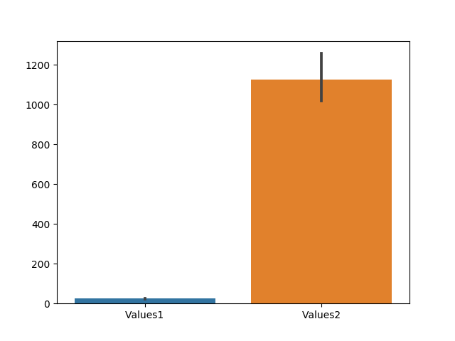
This doesn't give an idea about the comparison between the values of the two attributes. Now, let's normalize the values using the scikit package.

normalise:preprocessing.MinMaxScaler()
x:dataset[['Values2']].values.astype(float)
dataset['Values2']:normalise.fit_transform(x)
x:dataset[['Values1']].values.astype(float)
dataset['Values1']:normalise.fit_transform(x)

There, it is as simple as that. I am using min-max scaler just as an example. The preprocessing package offers more than one type of normalization functions.

Moving on, let's plot the graph now after normalization.

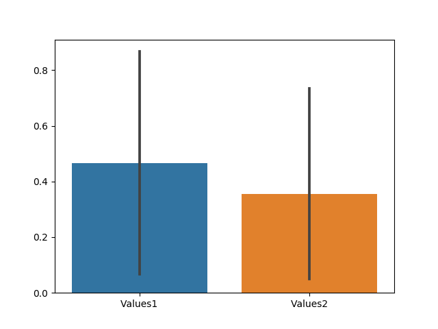
Drastically different, right?

The key is to play around and see what preprocessing functions are used on similar datasets. This might give you an idea of what can and can not be expected.

There, you have your processed dataset now. Have fun :P